| Figure 9.1. Postulated maximum areal extent of glacier ice in the north polar region during the Late Pleistocene Epoch (from Denton and Hughes, 1981a). |  |
|---|
Richard S. Williams, Jr.*
This chapter discusses the use of satellite images in examining selectively, on a global basis, the effect on the Earth´s surface of glaciers and glacial processes, especially the distribution and types of present-day glaciers, landforms resulting from glacial and fluvioglacial erosion and deposition during the Quaternary, and landforms resulting from active or relict periglacial processes. In many respects, this chapter is a space-age version of a similar review of glaciers and glacial landforms done by Shaler and Davis (1881) more than 100 years ago. Their pioneering work was one of the first publications to combine text with newly available ground photographs of glaciers and glacial landforms.
| Figure 9.1. Postulated maximum areal extent of glacier ice in the north polar region during the Late Pleistocene Epoch (from Denton and Hughes, 1981a). | |
|---|
A glacier is a mass of ice (>0.1 km2) that has its genesis on land and that represents a multiyear surplus of snowfall over snowmelt. According to Sugden and John (1976) and Flint (1971), perennial ice covers about 10 percent (1.5 x 10⁷ km2) of the land areas of the Earth (Table 9-l). Although glaciers are generally thought of as polar entities, as this table shows, they are also found in mountainous areas throughout the world, on all continents except Australia, and even at or near the Equator on high mountains in Africa, South America, and the East Indies.
| Geographic Region | Approximate Areea (km2) | Subtotals (km2) |
|---|---|---|
| South Polar Region | - | 12 588 000 |
| Antarctic Ice Sheet (excluding shelves) Other Antarctic Glaciers Subantarctic Islands |
**12 535 000 50 000 3 000 |
- |
| North Polar Region | - | 2 081 616 |
| Greenland Ice Sheet Other Greenland Glaciers Canadian Arctic Archipelago Iceland Spitsbergen and Nordaustlandet Other Artic Islands |
1 726 400 76 200 153 169 12 173 58 016 55 658 |
- |
| North American Continent | - | 76 880 |
| Alaska Other |
51 476 25 404 |
- |
| South American Cordillera | - | 26 500 |
| European Continent | - | 9 276 |
| Scandinavia Alps Caucasus Other |
3 810 3 600 1 805 61 |
- |
| Asian Continent | - | 115 021 |
| Himalaya Kun Lun Chains Karakoram and Ghujerab-Khunjerab Ranges Other |
33 200 16 700 16 000 49 121 |
- |
| African Continent | - | 12 |
| Pacific Region (including New Zealand) | - | 1 015 |
| Total | - | 14 898 320 |
Present-day glaciers and the deposits from more exten sive glaciation in the geological past have considerable economic importance in many areas. In regions of limited precipitation during the growing season, such as parts of the western United States, glaciers are considered to be frozen freshwater reservoirs that release water during the drier summer months. In some semiarid areas, glaciers are of considerable economic importance in the irrigation of crops. In mountainous areas such as Switzerland, Norway, and Iceland, meltwater from glaciers is critical to the economic generation of hydroelectric power. Lakes and ponds are numerous where continental ice sheets once covered vast areas of North America, Europe, and Asia (Figure 9-1), and the glacial deposits in these regions act as major ground-water reservoirs. These deposits also have substantial economic value as sand and gravel for construction and are often the basis, as in the Commonwealth of Massachusetts, for the largest mineral industry in a state.
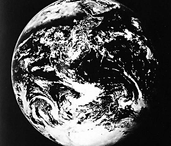 |
Figure 9.2. Apollo 17 photograph of the Earth showing most of the continent of Antarctica on the bottom of the globe. |
|---|
Within the past 3 million years, glaciers-in the form of ice caps and ice sheets-repeatedly expanded to cover about 29 percent (Flint, 1971) of the total land area of the Earth (Table 9-2). This land area includes most of Canada, all of New England, much of the upper Midwest, large areas of Alaska, most of Greenland, Iceland, Svalbard, other arctic islands, and Scandinavia, much of Great Britain and Ireland, and the western part of northern U.S.S.R. (Figure 9-1). Along mountainous coasts and high mountains of the interior in these areas, however, peaks and ridges would have protruded above the ice as nunataks. Parts of southern South America, central Asia, the Alps, and many other mountainous areas in Asia also experienced an increase in glacier extent. Glaciers in Antarctica likewise expanded somewhat, but more in ice thickness than in ice area because of the limiting effect of the surrounding oceans.
| Glaciated Region | Approximate Area (km2) |
Area Subtotals (km2) |
|---|---|---|
| South Polar Region | - | 13 810 000 |
| Antarctic Ice Sheet Sub-Antarctic Islands |
13 800 000 10 000 |
- |
| North Polar Region | - | 2 797 737 |
| Greenland Ice Sheet Iceland and Jan Mayen Island Spitsbergen and Nordaustlandet Other Arctic Islands |
2 295 300 142 000 298 662 61 775 |
- |
| North American Continent | - | 16 217 091 |
| Laurentide Ice Sheet Alaska Other |
13 386 964 1 033 062 1 797 065 |
- |
| South American Cordillera | - | 870 000 |
| European Continent | - | 6 721 708 |
| Scandinavian Ice Sheet Alps, Pyrenees, and other Continental Areas Caucasus |
6 666 708 39 000 16 000 |
- |
| AsianContinent | - | 3 935 000 |
| Himalaya and Other Mountains Outside
U.S.S.R. Ural/Siberian Ice Sheets Mountains in Northeastern U.S.S.R. Mountains in Southern U.S.S.R. |
189 000 2 707 000 707 000 332 000 |
- |
| Africa | - | 1 900 |
| Pacific Region | - | 30 000 |
| Total | - | 44 383 436 |
| Figure 9.3. Landsat RBV image of flow lines, creavasses, and nunataks on the lower part of the Rennick Glacier, Antarctica. | 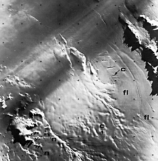 |
|---|
Although four or five major glacial advances have been identified by glacial geologists who have studied glacial deposits in Europe and North America, stratigraphic evidence from the Tjornes area of northern Iceland suggests that as many as 10 major glacial advances may have occurred within the past 3 million years or during what is popularly referred to as the Ice Age (Einarsson et al., 1967). On the basis of paleomagnetostratigraphic studies in southwestern Iceland, Kristjánsson et al. (1980) stated "that at least 13 glaciation occurred in western and southwestern Iceland between 3.1 and 1.8 Ma ago." The correlation of oxygen isotope ratios from deep-sea cores with the results of statistical analyses of the periodicity of the three astronomical elements of the Earth´s orbit confirmed the fact that many cycles of glacier advance and recession occurred during the Pleistocene (Imbrie and Imbrie, 1980).
At the present time, most of the glacial ice on the planet is encompassed in the two largest ice sheets, Antarctica (bottom of Figure 9.2) and Greenland (Figure G-1.3), which together contain an estimated 97 percent of all the glacial ice and 77 percent of the freshwater supply on Earth. During a maximum global advance of glaciers, however, it is estimated that North America contained volumetrically nearly as much ice as the present combined total of Antarctica and Greenland and that the sea level dropped by as much as 100 m (Flint, 1971).
Role of Satellite Surveillance in Glacial Studies
Until the launches in 1972, 1975, 1978, 1982, and 1984 of the five spacecraft in the Landsat series of Earth-resources satellites, glaciologists had no accurate means of measuring the areal extent of glacier ice on a global basis. Only Multispectral Scanner (MSS) images provided the worldwide coverage (except for the circular areas poleward of 81° north and south latitudes) needed for global geomorphological investigations. Coverage by higher resolution Landsat sensors (both TM and RBV at 30 m) has been more limited. Figure 9-3 is a Landsat-3 RBV image of the Rennick Glacier area of northern Victoria Land, Antarctica, showing the improved morphologic detail of many glaciological features: flow lines (fl), crevasses, (c), and nunataks (n), as compared with Landsat MSS images.
 |
Figure 9.4. A 1000-year history of variations in Iceland´s temperature compiled by various investigators from both proxy (historical records, chiefly old annals) and modern (thermometric) records (CIA, 1974, 1978: Thoroddsen, 1916, 1917. |
|---|
Landsat images provide a means for delineating the areal extent of ice sheets and ice caps, for determining the position of the termini of valley, outlet, and tidal glaciers, and for measuring the average speed of flow of some glaciers by a time-lapse method of sequential images on a common base of data for the entire globe. To take advantage of the vast amount of Landsat data of the glacierized regions of the planet, the U.S. Geological Survey (USGS), in association with more than 50 United States and foreign glaciologists and glacial geologists, is working on a project to prepare a satellite image atlas of glaciers of the world (Williams and Ferrigno, 1981). If Landsat-type surveys of the Earth are continued for several decades, a means of monitoring long-term changes in glacier area will also become possible, thereby providing means for monitoring one potential effect of global climatic change (Williams and Svensson, 1983a; Williams, 1985).
Because of their availability for most of the land areas of Earth, Landsat images are the primary source of image data for this chapter. Most images or photographs acquired by manned spacecraft are concentrated in the low or middle latitudes because of the restricted orbital inclination of most manned spaceflight missions conducted by the United States. The orbital inclination of Skylab, for example, reached about as far north or south as any manned mission-to 50° north and south latitude-and more than 35 000 photographs and images were acquired during the three occupations of the Skylab space station during 1973 and 1974 (Southworth, 1983). The Synthetic Aperture Radar (SAR) on board Seasat operated intermittently from late June until early October 1978 in an orbit that reached to a maximum of 72° north and south latitude. During two missions, the Space Shuttle has acquired two large sets of Shuttle Imaging Radar data-SIR-A and SIR-B. Seasat SAR (Ford et al., 1980) and Shuttle SIR data, with pixel sizes up to 25 m, produced some excellent images of glaciers and glacial landforms. Some of the Seasat SAR images appear in this chapter.
| Figure 9.5. Landsat false-color (special) composite image of Vetnakökull, Iceland, showing the accumulation and ablation areas on the ice cap. |  |
|---|
The great value of image data acquired from Earth-orbiting spacecraft is that it gives scientists the capability to study and to monitor our planet on a global basis. In particular, the Landsat series has markedly broadened the availability of image data of the Earth´s surface, so that geomorphologists now have two-dimensional image information of virtually the entire land area and many shallow sea areas of the planet. Local and regional geomorphological studies carried out since the 1930s have traditionally used stereopairs of vertical aerial photographs because of the analytical importance of viewing landforms in three dimensions, rather than two. Generally speaking, most satellite images portray the Earth´s landforms in two dimensions, although low solar-angle illumination of the terrain can often provide an illusion of the third dimension. In many cases, the geomorphic analysis of landforms on satellite images in only two dimensions can be a drawback. Another drawback in the analysis of landforms on satellite images is that, on Landsat MSS images, for example, only landforms large enough to be represented by a few pixels can even be detected, and tens of pixels are needed for identification. As a result, many types of landforms are simply not visible on Landsat images. In unknown or unfamiliar regions, the scientist using such images may not even be aware of what is "missing." For example, in a recent paper on Icelandic volcanoes, 27 discrete types of volcanoes can be identified in Iceland on vertical aerial photographs (Williams et al., 1983b), and only 6 of the 13 types of Icelandic basaltic volcanoes previously described by Thorarinsson (1959) could be unambiguously recognized on Landsat images (Williams et al., 1974).
It is important for geologists who use Landsat images for geomorphological, structural, tectonic, and other types of geological investigations to be aware of the limitations of such images, especially in the two-dimensional and in the spatial resolution aspects. The 26 Plates showing glaciers, glacial landforms, and periglacial landforms in this chapter describe features that are large enough to be delineated on Landsat or other types of satellite images and can be well portrayed in two dimensions.
Glaciers form in any area in which a year-to-year surplus of snow occurs. Under such conditions, successive layers of snow are slowly compacted until the loose snowflakes form a monomineralogic (frozen H2O) sedimentary deposit that gradually becomes more and more dense with increasing depth and age. When a density of 830 to 910 kg/m3 is reached, formation of ice occurs (Paterson, 1981). As the effect of gravity slowly deforms this mass of ice, a glacier is formed. A glacier therefore represents an unusual type of metamorphic rock, being the result of deformation of what was originally a sedimentary rock.
Glaciers are of considerable scientific interest because of the extensive record of variations in atmospheric gases and aerosols contained within a vertical column of glacier ice. In optimum geographic locations, the record can extend over several hundred thousand years and provide specific information about variations in carbon dioxide (CO2), the O18/O 16 ratio (a measure of temperature in the lower atmosphere), variations in meteoritic infall rates, the occurrence of explosive volcanic activity through deposition of tephra, etc. The impact of the industrial revolution on the Earth´s surface and atmosphere can also be determined through careful analyses of cores of glacier ice.
The fluctuation of glaciers, especially fluctuations in volume of glacier ice, is related to climatic variations (Williams, 1983d). Although the historical record of glacier fluctuation is not very lengthy in most glacierized regions, glaciers were known to have advanced during what is known as the "Little Ice Age" (the period from the late 1500s to the late 1800s). There has been a general retreat of glaciers since the late 1800s until the late 1950s or early 1960s. Perhaps the best record of variation in climate during the past 1000 years is the proxy record of the mean annual change in Iceland´s temperature compiled from Icelandic sources by various investigators ( Figure 9-4; CIA, 1974, 1978). The later temperature record for Iceland shown in Figure 9-4 is from actual thermometric measurements. The glaciers of Iceland, several of which are used to illustrate glaciers, glaciological phenomena, and glacial landforms in this chapter, are of special value to understanding the link between climatic change and glacier fluctuation. At about 64° north latitude, Iceland´s glaciers are especially sensitive to the climatic variation resulting from secular changes in the Earth´s orbital history (eccentricity, tilt, and precession), which form the basis for the Milankovitch theory of glacier advance and recession (Imbrie and Imbrie, 1980).
| Reservoir | Percentage of Total Water Supply by Volume |
|---|---|
| Surface Water | (1.71 x 10⁻²) |
| Freshwater Lakes Saline Lakes and Inland Seas Average in Stream Channels |
9 x 10⁻³ 8 x 10⁻³ 1 x 10⁻⁴ |
| Subserface Water | (6.25 x 10⁻¹) |
| Vadose Water (includes soil
moisture) Ground Water (within upper 0.8 km of the Earth´s crust) Ground Water (deeper than 0.8 km) |
5 x 10⁻³ 3.1 x 10⁻¹ 3.1 x 10⁻¹ |
| Other | (99.351) |
| Glacier Ice Atmosphere Oceans |
2.15 1 x10⁻³ 97.2 |
| Total | 100 |
As previously discussed, 10 percent of the present land area of our planet is covered by glacier ice. Glaciers comprise 2.15 percent of the total water supply of the planet, the second largest "reservoir" after the Earth´s oceans, which are the biggest repository at 97.2 percent (Table 9-3). Glacier ice is represented by a special class of landforms called glaciers. Glaciers range in size from about 0.1 (Meier, 1974) to 13 586 380 km2 (Antarctic ice sheet including ice shelves) (Drewry et al., 1982) and have been classified into several well-defined groups on the basis of morphology and physiographic setting. A glacier classification and description scheme (Table 9-4) was developed by the International Association of Scientific Hydrology (IASH) in 1970 (UNESCO, 1970) for use in a computerized data archive for the World Glacier Inventory Project (Müller et al., 1977). The IASH classification and description guidelines are especially useful when using aerial photographs or satellite images to assist in determining the six parameters of a glacier.
 |
Figure 9.6. Schematic diagram of the subdivisions of the accumulation zone of a glacier (from Paterson, 1981). |
|---|
Meier (1974) discussed three main types of glaciers: (1) continuous masses of ice moving outward in all directions, such as ice sheets or their much smaller counterparts, ice caps; (2) linear masses of ice constrained in their flow by topography, such as outlet glaciers, valley glaciers, cirque glaciers, and ice streams; and (3) cake-like masses of ice that spread laterally on level ground or in coastal areas, such as piedmont glaciers and ice shelves. Examples of each of these types of glaciers are presented in the Plates section. Two special subtypes of glaciers are also included- surging glaciers and tidal glaciers-because of the special effect they can have on modifying the preglacial landscape.
| - | DIGIT 1 Primary classification |
DIGIT 2 Form |
DIGIT 3 Frontal characteristic |
DIGIT 4 Longitudinal profile |
DIGIT 5 Major source of nourishment |
DIGIT 6 Activity of tongue |
|---|---|---|---|---|---|---|
| 0 | Uncertain or misc. |
Uncertain or misc. |
Normal or misc. |
Uncertain or misc. |
Uncertain or misc. |
Uncertain |
| 1 | Continental ice sheet |
Compound basins |
Piedmont | Even: regular | Snow and/or drift snow |
Marked retreat |
| 2 | Ice field | Compound basin | Expanded foot |
Hanging | Avalanche ice and/or avalanche snow |
Slight retreat |
| 3 | Ice cap | Simple basin | Lobed | Cascading | Superimposed ice |
Stationary |
| 4 | Outlet glacier | Cirque | Calving | Icefall | - | Slight advance |
| 5 | Valley glacier | Niche | Coalescing noncontributing |
Interrupted | - | Marked advances |
| 6 | Mountain glacier | Crater | - | - | - | Possible surge |
| 7 | Glacieret | Ice aprons | - | - | - | Known surge |
| 8 | Ice shelf | Groups of small units |
- | - | - | Oscillating |
| 9 | Rock glacier | Remnant | - | - | - | - |
| - | ||||||
| Digit 1 Primary Classification | ||||||
| 0 | Miscellaneous | Any not listed | ||||
| 1 | Continental ice Sheet | Inundates areas of continental size. | ||||
| 2 | Ice field | Ice masses of sheet or blanket type of a thickness not sufficient to obscure the subsurface topography. | ||||
| 3 | Ice cap | Dome-shaped ice mass with radial flow. | ||||
| 4 | Outlet glacier | Drains an ice sheet or ice cap, usually of valley glacier form; the catchment area may not be clearly delineated. | ||||
| 5 | Valley glacier | Flows down a valley; the catchment area is well defined. | ||||
| 6 | Mountain glacier | Cirque, niche, or crater type; includes ice aprons and groups of small units. | ||||
| 7 | Glacieret and snowfield |
A glacieret is a small ice mass of indefinite shape in hollows and river beds and on protected slopes developed from snow drifting, avalanching, and/or especially heavy accumulation in certain years; usually no marked flow pattern is visible and therefore no clear distinction from snowfield is possible. Exits for at least two consecutive summers. | ||||
| 8 | Ice shelf | A floating ice sheet of considerable thickness attached to a coast, nourished by glacier(s); snow accumulation on its surface or bottom freezing | ||||
| 9 | Rock glacier | A glacier-shaped mass of angular rock in a cirque or valley either with interstitial ice, firn, and snow or covering the remnants of a glacier, moving slowly downslope. | ||||
Glaciers are a peculiar type of landform because they can in turn modify the existing (preglacial) landscape, producing both erosional and depositional landforms. The process by which a glacier modifies the subglacial and adjacent landscape is by the action of moving ice and by the deposition of till beneath and adjacent to the glacier. Glaciers also affect areas peripherally by discharging large amounts of sediment-laden meltwater. Some of the eolian deposits, called loess, are produced from erosion and redeposition of fine-grained sediment derived from glacial outwash. Erosion and deposition can also result from catastrophic outburst floods (jökulhlaups) caused by the failure of ice-dammed lakes or, more rarely, from subglacial volcanic eruptions or geothermal activity. The cold climate adjacent to glaciers usually fosters periglacial processes that produce special types of landforms as the result of the action of ground ice, including an unusual type of "glacier" composed of rock fragments and ice. Such a glacier is called a rock glacier.
| Figure 9.7. Oblique, aerial photograph of the margin of Sídujökull, an outlet glacier from Vatnojökull, Iceland. | 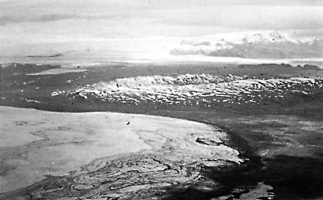 |
|---|
Three special-topics dealing with glaciological phenomena that have proven to be especially amenable to delineation on Landsat images are included in this section of the introduction: the accumulation zone of a glacier, areas of blue ice in Antarctica, and subglacial volcanoes.
Glacier Mass Balance
The mass balance of a glacier is defined by Bates and Jackson (1980) as: "The change in mass (the difference between total accumulation and gross ablation) of a glacier over some defined interval of time, determined either as a value at a point, an average over an area, or the total mass change for the glacier. The units normally used are millimeters, meters, or cubic meters of water equivalent, but kilograms per square meter or kilograms are used by some." Mass-balance studies of glacier provide a measure of its condition. Is it gaining (positive) or losing (negative) mass? There are several ways to determine the mass balance of a glacier (Paterson, 1981), but all are labor-intensive and costly. As a result, the records of very few glaciers contain their mass balance in 1 year or over several years.
Studies of the Greenland Ice Sheet by Benson (1962) and of the ice caps and outlet glaciers of Axel Heiberg Island, Northwest Territories, Canada, by Müller (1962) led to the development of the concept of zonation of the accumulation zone of temperate glaciers and the relationship between the accumulation zone, firn line, equilibrium line, and ablation zone. If one can determine the late summer season snowline, which is a good approximation of the equilibrium line on temperate glaciers (Paterson, 1981), then the accumulation area ratio-the area of the accumulation area at the end of summer divided by the glacier´s area-can be determined. As noted by Glen (1963) in Paterson (1981), "A rule of thumb is that an accumulation area ratio of about 0.7 corresponds to a net balance of zero." This means that aerial photographs and satellite images, if acquired at the optimum time in late summer, can be used to determine the accumulation area ratio of temperate glaciers. In fact, (Østrem (1975) directly applied this concept to Landsat images of Norwegian glaciers. Østrem´s work is an extension of the previous research by Meier and Post (1962), who first described the use of equilibrium line altitudes and accumulation area ratios, derived from aerial photographs, to infer the regional distribution of glacier mass balances.
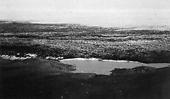 |
Figure 9.8. Oblique aerial photograph of the margin of Brúarjökull, a broad, surging outlet glacier from Vatnajökull, Iceland. |
|---|
Figure 9-5 is a Landsat MSS false-color composite image (1426-12070; September 22, 1973) of Vatnajökull ice cap and environs, Iceland. MSS bands 5, 6, and 7 were enhanced by special computer processing and were projected through yellow, red, and blue filters, respectively, to create a false-color composite image. The original computer- generated histograms of the spectral characteristics of the image fell into three groupings (trimodal), thereby permitting snow-covered areas, vegetation, and bare rock or soil to be processed independently. Each of these zones was stretched in each of the three MSS bands to encompass the full range of brightness and was then composited by the Image Processing Laboratory of the California Institute of Technology´s Jet Propulsion Laboratory (Soha et al., 1976). This type of computer-enhanced image of Vatnajökull (see also Plate G-6 for a standard Landsat false-color composite of Vatnajökull) appears to provide a good correlation of glacier color with the zones in the accumulation area and the ablation area shown schematically in Figure 9-6, a schematic representation of the zones in the accumulation zone of a glacier, the area up-glacier from the equilibrium line. Bare glacier ice is exposed down-glacier (to the right of the firn line in that figure). The ablation zone extends down- glacier from the equilibrium line (see Figure 9-5; from Björnsson, 1971, after Paterson, 1969, 1981). The concept of zonation in the accumulation area was developed by Benson (1962) from his work in Greenland and by Müller (1962) from his work on Axel Heiberg Island, Northwest Territories, Canada. On Vatnajökull, the colors apparently correlate as follows: light blue, the bare glacial ice of the ablation zone; orange, superposed ice, including the approximate position of the equilibrium line; black, soaked zone; dark gray, percolation zone; light blue-gray, dry-snow zone (Williams, 1983c).
| Figure 9.9. Oblique aerial photograph of the oblation zone of Brúarjökull, Iceland, showing contorted tephra layers and supraglacial drainage. | 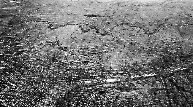 |
|---|
Figure 9-7, an oblique aerial photograph (taken on August 17, 1973) of the terminus of Sídujökull, one of the outlet glaciers on the southwestern margin of Vatnajökull, shows the bare glacial ice of the ablation zone (see Figure 9-6) in the foreground. Last winter´s snow, now mostly firn, is visible at higher elevations of the glacier lobe. Note the patterns produced by the ablation surface cutting across ice foliation (complex patterns of ice deformation outlined by tephra layers and seasonal dust layers due to flow processes up-glacier). At the end of the summer season, the demarcation between the bare ice and firn- covered ice is the approximate position of the equilibrium line on temperate glaciers. Figure 9-8 and Figure 9-9 are a pair of oblique aerial photographs (taken on August 17, 1973) of another outlet glacier coming off Vatnajökull, Brúarjökull (see Plate G-10), that show the ablation zone from a different perspective. Figure 9- 8, a high-angle oblique photograph, depicts a proglacial lake in the foreground, bare ice of the ablation zone in the middle background, and last winter´s snow cover in the background. Figure 9-9, a low- angle oblique, shows bare glacial ice in the foreground with a supraglacial stream valley and channel in the foreground, the complex ice-fracture patterns, and wavy patterns of deformed tephra layers. Last winter´s snow cover is visible in the far background. An August 1978 Landsat-3 RBV image of Brúarjökull that illustrates the transient snowline dividing the accumulation zone from the ablation zone is shown on Plate G-16.
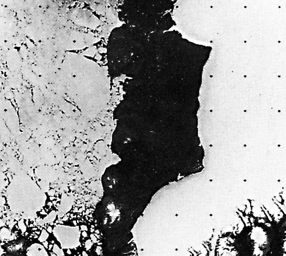
Blue Ice
The term "blue ice" was introduced by the late Swedish glaciologist, Valter Schytt, during observations made on the 1949-1952 Norwegian/British/Swedish Antarctic Expedition to Queen Maud Land (V. Schytt, January 6, 1983, private communication; Schytt, 1961). He used the term to refer to areas of bare glacier ice. Such areas of blue ice primarily occur near the coast and in interior areas both upstream and downwind from nunataks, the peaks of mostly buried mountain ranges or isolated massifs. Blue ice is caused by ablation, which results mainly from sublimation, wind-scouring of the snow mantle, and surface polishing by wind-driven snow (Williamset al., 1983a). Bare glacial ice or blue ice also occur extensively in Greenland, especially during mid- to late summer, when the previous winter snowfall has melted from the margins of the ice sheet. Although much more limited areally, blue ice is also characteristic of the lower parts of valley and outlet glaciers and along the margins of ice caps in late summer.
 |
Figure 9.10a. Landsat image of the Queen Fabiola (Yamato) Mountain area, East Antarctica, showing extensive areas of "blue ice" (bare glacier ice) around nunataks and associated morainal debris. |
|---|---|
 |
Figure 9.10b. Index map showing selected geographic, geomorphic, and glaciological features on Figure 9-10a. |
The term "blue ice" has special significance in Antarctica, however. Since 1969, more than 6000 fragments of meteorites, including at least 600 individual meteorites,have been discovered in blue- ice areas of Antarctica. Many of these meteorite finds have included types that are exceedingly rare (Marvin, 1984), and the full suite of specimens so far discovered provides an extraordinarily fine representation of the range of meteorite types that have reached the Earth´s surface. Therefore, Antarctica has become the most important collecting area on our planet for meteorites.
Brown (1961) estimated the Earth´s meteorite infall rate to be approximately one per square kilometer each million years. Basing his work on this figure, a model of the East Antarctic ice sheet, and other factors, Olsen (1981) estimated that at least 760 000 meteorites are likely to lie in the East Antarctic ice sheet. Most of those recovered to date in Antarctica have been found in areas of blue ice, especially around nunataks or where the normal flow of glacier ice is impeded or stopped.
| Figure 9.11. Photograph of blue-ice area in west Antarctica. | 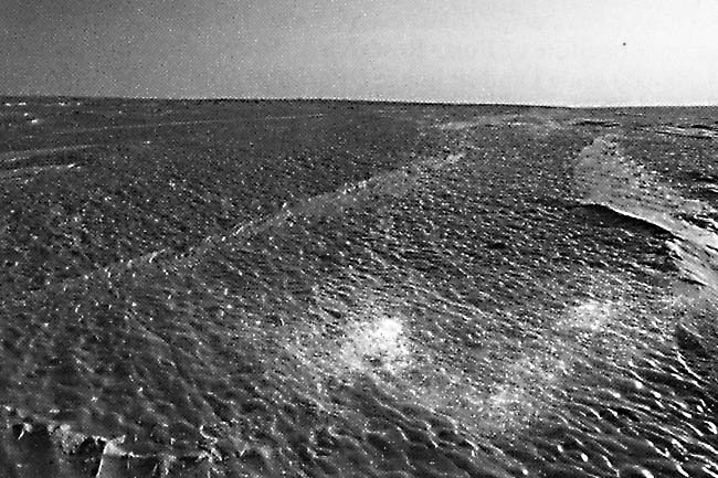 |
|---|
A U.S. Geological Survey colleague, Mark F. Meier (written communication, 1982), noted that ". . . meteorite concentrations pose interesting glaciological problems: I would expect that the highest concentrations would be found in areas combining high vertical strain rates with high ablation rates; areas of high strain rates might be predictable from the flow geometry, which might be identifiable on Landsat imagery." He also noted that the greater the ablation, the greater the volume of ice that would flow through meteorites. Thus, it is likely that concentrations of meteorites will be found in areas of blue ice, which can be identified not only from surface traverse and aerial reconnaissance, but also by systematic search of satellite imagery.
The launch of Landsat-1 in July 1972 provided the first opportunity for higher resolution satellite image coverage of Antarctica. Excellent Landsat images of the Queen Fabiola (Yamato) Mountains were acquired as early as December 1973. Later, the National Institute of Polar Research in Tokyo, Japan, published a 1:200 000- scale Landsat image (Working) Map of the Meteorite Ice Field, Yamato Mountains, Antarctica (1976), which delineated areas of blue ice, nunataks, morainal debris, and spot elevations derived from ground surveys. In the identification of blue ice areas, MSS bands 6 and 7 are similar, with band 7 somewhat better than MSS band 6. MSS band 5, however, is best in areas of bedrock exposure (e.g., nunataks) for proper differentiation between areas of blue ice and either bedrock or morainic debris. On MSS bands 6 and 7, blue ice and rock usually have a similar spectral response. Mark F. Meier (written communication, 1982) suggested experimenting with computer-assisted analysis of different MSS bands because blue ice should be distinctive enough (spectrally) for a computer to identify with high accuracy (Williams et al., 1983a). Figure 9-10a and Figure 9-10b are a Landsat- 1 MSS false-color composite and its index map that cover the Queen Fabiola (Yamato) Mountains area, East Antarctica, which displays extensive areas of blue ice (bare glacier ice) around nunataks and associated morainal debris. Landsat (and NOAA) images can be used to delineate areas of blue ice in Antarctica, some of which have proved to contain extraordinary accumulations of meteorites. Since 1969, Japanese scientists have collected 4813 meteorites within the blue-ice areas shown on this image or about 25 percent of the extant worldwide collection of meteorites.
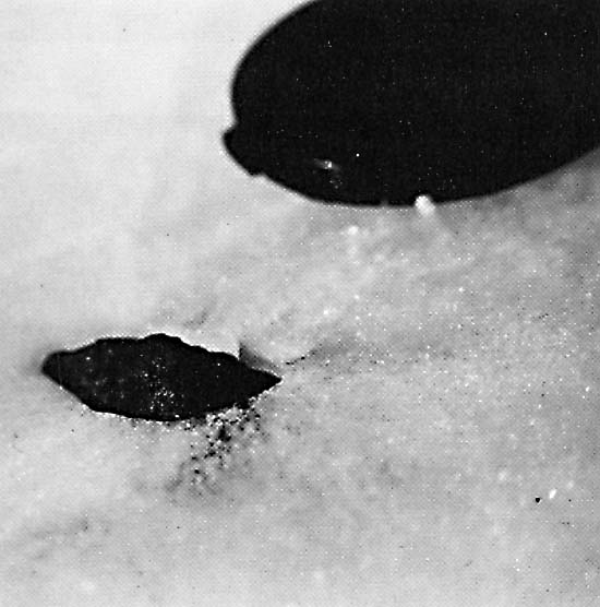 |
Figure 9.12. Photograph of chondritic meteorite emerging at the ice-sheet surface, Allan Hills, Antarctica. |
|---|
During the 1982-1983 field season, a meteorite-collection effort in blue-ice exposures of the Allan Hills/ "Elephant Moraine" areas of Victoria Land, West Antarctica, used a Landsat image to identify areas of blue ice, to plot traverses through and between blue-ice patches, and to locate collection points in a general sense. Precise geographic positions were established with a Magnavox Model MX1502 geoceiver in conjunction with overpasses of the Navy navigational satellite system (Cassidy et al., 1984; Williams et al., 1984). Meteorites were collected from each of the blue-ice areas identified on the Landsat image and were actually viewed in the field (T. K. Meunier, private communication). Figure 9-11 is a photograph of the cupped and scalloped surface of the blue ice in the "Elephant Moraine" area, Victoria Land, West Antarctica. Figure 9-12 shows the only meteorite so far recovered in situ within blue ice in Antarctica. This H-5 chondrite (ALH-82102) weighed 48 g (35-mm camera lens cap indicates scale). Figure 9-13 is a large H-5 chondrite (ALH-82103) that weighed 2.53 kg. This meteorite was one of the largest of the 113 collected during the 1982- 1983 field season.
Subglacial Volcanoes
In volcanically active regions with an extensive cover of glacier ice, volcanoes may be wholly or partly subglacial. Volcanoes and glaciers often coexist because areas of extensive volcanic activity tend to be regions of higher than normal elevation. Glacier-shrouded volcanoes with a history of volcanic activity include several volcanoes in Iceland; Mount Beerenberg on Jan Mayen (Island), Norway; Mount St. Helens (Plate V-8) (Brugman and Post, 1982) and other volcanoes of the Cascade Mountains, northwestern United States; numerous volcanoes in Alaska, both on the mainland and along the Aleutian Islands arc (Plate V-9) (Post and Mayo, 1971); volcanoes on the Kamchatka Peninsula, U.S.S.R. (Plate V-25); and volcanoes in the Andes Mountains (including the Patagonian Ice Field) of South America (Plate V-14) and in Antarctica.
| Figure 9.13. Photograph of large chondritic meteorite on the ice sheet surface, Allan Hills, Antarctica. | 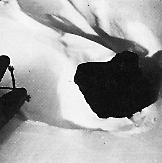 |
|---|
The eruption of a volcano under a glacier can produce a catastrophic outpouring of enormous quantities of water melted from the ice by the thermal energy. Perhaps best known from repeated occurrences in Iceland, where glacial-outburst floods are known as jökulhlaups, such extraordinary discharges of water represent a powerful geomorphic agent in regions in which glaciers and volcanoes coexist. Two ice caps in Iceland have had a lengthy historical record of jökulhlaups resulting from subglacial volcanic and/or geothermal activity and volcanic activity, respectively: Vatnajökull (Plate G-6) and Myrdalsjökull ( Plate G-22). Jökulhlaups from the Grímsvötn caldera (see Plate G-15, Figure 9-14, and the index map for Plate G-6) in the west-central part of Vatnajökull produced floods in the 50 000 m3/s range several decades ago, but have dropped to the 10 000 m3/s in recent years because of apparent thinning of the ice cap around the caldera (Björnsson, 1975; Tómasson, 1975). Figure 9-14 is an oblique aerial photograph of the 45-km2 subglacial/subaerial caldera looking toward the east. Most of the jökulhlaups originating in the Grímsvötn caldera occur as the result of the lifting of the ice dam on the east side of the caldera whenever the subglacial lake in the caldera fills to a certain level. The input of water to the closed subglacial basin is believed to be from the melting of ice by subglacial geothermal activity and from seasonal ablation rather than in association with a volcanic eruption. The volcano Katla, which is located under the eastern part of Myrdalsjökull (Plate G-22), was estimated by Thorarinsson (1957) to produce floods in excess of 100 000 m3/s and perhaps as high as 200 000 m3/s from eruptions. Other sites within Vatnajökull have also produced jökulhlaups from periodic volcanic and/or geothermal activity: Öraefajökull (Thorarinsson, 1956b) Kverkfjöll (Friedman et al., 1972), and the collapse caldrons east of Hamarinn (Plates G-6 and G-15) (Thorarinsson et al., 1974).
| Figure 9.14. Oblique aerial photograph of the Grímsvötn subglacial/subaerial volcanic caldera, west-central Vatnajökull, Iceland. | 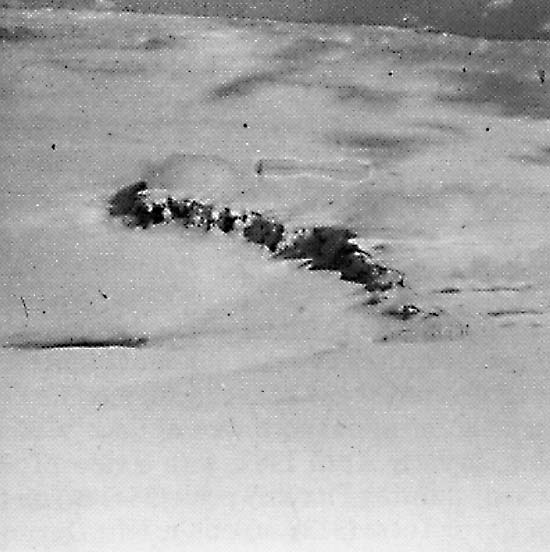 |
|---|
Landsat images are especially well suited to show the morphology of large glacier-capped or glacier-shrouded volcanoes. Morphological changes on the surface of ice caps caused by subglacial volcanic and/or geothermal activity can also be well studied, if of large enough dimensions (Thorarinsson et al., 1974; Björnsson, 1975, 1976: and Tómasson, 1975) (see also Plates G-6 and G-15).
The continent of Antarctica and nearby offshore islands contain a number of volcanoes, only five of which are considered to be active (Simkin et al., 1981): the three stratovolcanoes-Mount Melbourne (in northern Victoria Land), Mount Berlin (in Marie Byrd Land), and Mount Erebus (on Ross Island; see Plate G-l)-and the two calderas-Mount Hampton (in Marie Byrd Land) and Deception Island (near the tip of the Antarctic Peninsula). The volcanoes of Buckle Island in the Balleny Islands, Penguin Island, Paulet Island, and Lindenberg Island are also considered to be active on the basis of field studies (Simkin et al., 1981). Mount Erebus and Deception Island have historically been the most active, with at least 10 eruptions documented for each (Simkin et al., 1981).
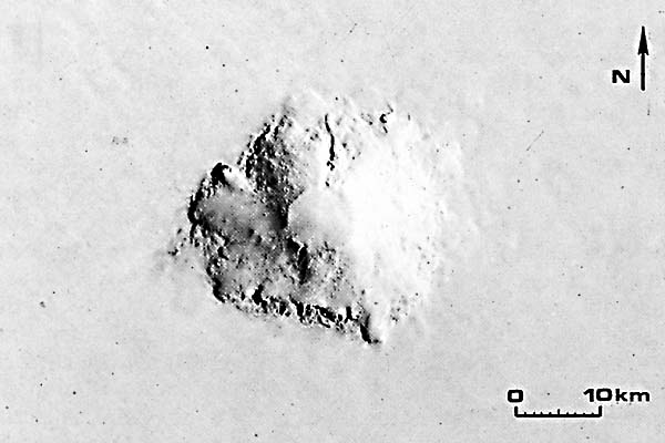 |
Figure 9.15. Landsat image of Mount Takahe, a partially buried shield volcano, West Antarctica. |
|---|
A number of volcanoes in Antarctica have no known record of historic activity, but have well-developed summit craters or calderas. A variety of such volcanoes occur in West Antarctica in Marie Byrd Land between about 110 and 140°W longitude, either as isolated mountains or as a group of volcanoes within a mountain range. Landsat images are of particular value in providing two-dimensional morphological information on these volcanoes in West Antarctica.
Figure 9.15 is an enlarged part of a Landsat image of Mount Takahe volcano, which is centered at about 76°15´ south latitude, 112°05´ west longitude. Mount Takahe is a partially buried shield volcano, approximately 30 km in diameter and topped by an 8-km wide quasi-circular caldera. The highest elevation within the caldera is about 3460 m, and the surface elevation of the Antarctic ice sheet at the base of the volcano is about 1200 m (U.S. Geological Survey, 1976a). Figure 9.16 is an oblique (trimetrogon) aerial photograph of Mount Takahe, the type of data used by the U.S. Geological Survey to prepare the 1:250 000 scale (Reconnaissance Series) maps of Antarctica.
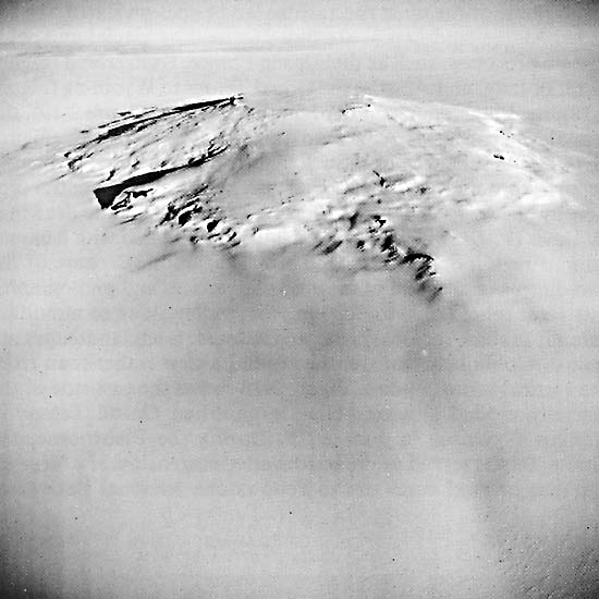 |
Figure 9.16.Oblique aerial photograph of Mount Takahe valcano in West Antarctica. |
|---|
Subglacial volcanic eruptions produce specialized types of landforms caused by the interaction of molten rock and meltwater from the surrounding glacier and the encapsulation of the volcanic activity by the glacier ice. In Iceland, where landforms formed from subglacial volcanic activity abound, two distinct types can be recognized: (1) landforms resulting from central eruptions of basaltic lava, and (2) landforms resulting from linear eruptions of basaltic lava (Williams et al., 1983b). Volcanic landforms formed in this way are composed of hyaloclastite breccias and pillow lavas, characteristic of the so-called Móberg Formation in Icelandic. The linear landforms are called subglacial or móberg ridges, especially well depicted on Plate G-15 in the region between the southwestern part of Vatnajökull and the northeastern part of Myrdalsjökull. The subglacial landform that results from a subglacial eruption is called a table mountain ("stapi" in Icelandic). Figure 9.17 is an oblique aerial photograph looking across the 1961 lava flows from the Askja caldera toward the prominent Herdubreid table mountain in north-central Iceland. Table mountains, such as Herdubreid in northeastern Iceland, often perforate the overlying ice sheet in the last phase of their development, thereby producing a normal subaerial lava-shield landform as a cap on a socle of hyaloclastite breccias and pillow lavas. In the case of Herdubreid, the base of the lava shield stands about 1000 m above the surrounding terrain and represents the thickness of the Pleistocene ice sheet in that part of Iceland when Herdubreid formed. Icelandic table mountains are the subglacial/subaerial counterparts of subaerial lava-shield volcanoes (Williams et al., 1983a). With Herdubreid as an example, it is easy to imagine what Mount Takahe (Figures 9-15 and 9-16) would look like if the surrounding ice sheet were to melt away.
| Figure 9.17. Oblique aerial photograph of Herdubreid, a prominent table mountain in north-central Iceland. | 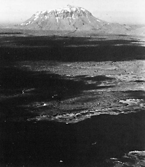 |
|---|
EROSIONAL GLACIAL LANDFORMS
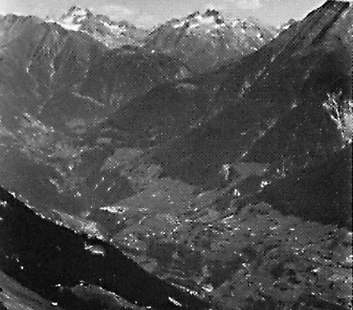
Some of the most spectacular landscapes on Earth, the so-called Alpine landscapes, are those formed by glacial and cold-climate processes, such as the Alps in France, Switzerland (Figure G-13.3), Italy, and Austria; the Grand Tetons in Wyoming (Figure 9.18), the Patagonian region of South America (Figure 9.19), the Himalaya in central Asia, and the fjords of Norway (Figure G-14.3) and other regions. Such landscapes derive their intrinsic beauty from the great local relief, the result of differential erosion by glacier ice. Figure 9-20 includes two schematic drawings by Davis (1909), which illustrate features associated with a mountainous region both during and after glaciation. Because of the two-dimensional aspect of most satellite images and photographs, this great relief (2000 to 3000 m from valley floor to mountain summit in some regions) is not appreciated. Such landscapes are best seen obliquely or from the ground aspect rather than from the vertical vantage point. Figure 9-18 shows the east side of the glacially eroded and cold-climate modified Grand Tetons in western Wyoming in June 1975. During the Pleistocene, the Grand Tetons served as the southwestern extension of a large ice cap that covered much of the Yellowstone National Park area, and the highest elevations probably protruded above the glacier as nunataks. Only small glaciers remain today in cirques on the uppermost flanks of this mountain range. Figure 9-19 shows the glacially eroded and cold-climate-modified Fitz Roy/Torre massif (granitic intrusion) northwest of Lago Viedma; Patagonia, Argentina, in early April 1982, with a view of the eastern side of the massif showing Fitz Roy peak (3441 m) on the right and the spire of Cerro Torre (3128 m) on the left. During the Pleistocene, this region was covered by a large ice cap that extended along the southern Andes Mountains (see Figure G-4.2).The angular ridges (arêtes) and spires (horns) probably rose above the ice cap as nunataks. Examples from space of cirques, arêtes, glacial troughs, and fjords are presented in Plates G-12, G-13, G-14, and G-26.
| Figure 9.18. Photograph of the east side of the glacially eroded Grand Tetons in western Wyoming. | 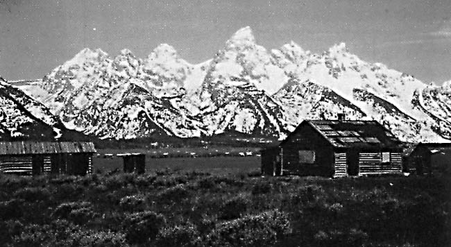 |
|---|
Except for glacial outburst floods (jökulhlaups), landforms resulting from glaciofluvial erosion are generally too small to be characterized on satellite images. One example of landscape modification from such a catastrophic process, the Channeled Scabland of eastern Washington, is included in Chapter 4, Fluvial Landforms (Plate F-27).
DEPOSITIONAL GLACIAL LANDFORMS
In the erosional process of modifying the preglacier landscape by glacier ice and running water, glaciers pick up, carry, and deposit vast quantities of fragmental material derived from the underlying surficial deposits, including deposits from previous glaciation, and bedrock. This fragmented material ranges from large blocks, often several to tens of meters in dimension, that are directly transported by glacier ice to very fine-grained material, called rock flour, that is transported in glacial streams or deposited directly from the glacier as a till matrix. On Landsat MSS false-color composite images, the color of proglacial lakes and streams that originate at glacier termini is a very characteristic robin´s-egg blue, indicating the presence of glacial rock flour in suspension. The outwash plain (sandur) or valley floor downstream from the terminus of a glacier, when dry, becomes the source for downwind deposits of eolian material called loess.
| Stratified Drift | Unstratified Drift |
|---|---|
| Ice-contact deposits | Lodgement till (ground moraine) |
| Proglacial deposits | Ablation till (terminal, recessional, lateral, and ground moraine) |
| Lacustrine deposits | Pressure or squeeze till |
| Undermelt deposits | Push till (moraine) |
Many varieties of landforms result from subglacial, supraglacial, and marginal processes associated with glacial and glaciofluvial deposition. Table 9-5 is a classification scheme for glacial and glaciofluvial deposits developed by Embleton and King (1975a).
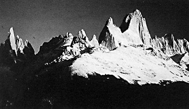 |
Figure 9.19. Photograph of the ice-modified Cerro Torre massif in Patagonia, Argentina. |
|---|
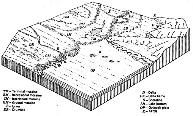
Morainic landforms have been intensively studied by glacial geologists as relict landform features of the Pleistocene Epoch (Prest, 1968) and as active landforms associated with present-day glaciers. Figure 9.21, modified from Flint (1971), shows the characteristic morainic, till, and other landforms resulting from glacial and glaciofluvial processes associated with a valley or outlet glacier. Till is defined by Bates and Jackson (1980) as "dominantly unsorted and unstratified drift, generally unconsolidated, deposited directly by and underneath a glacier without subsequent reworking by meltwater, and consisting of a heterogeneous mixture of clay, silt, sand, gravel, and boulders ranging widely in size and shape." Till has replaced the now obsolete term, "ground moraine." Table 9-6, a classification scheme developed by Ritter (1978), shows a variety of morainal landforms.
| End Moraines Terminal moraines |
Moraines produced at front or sides of an actively flowing
glacier. Mark the farthest advance of an important glacial episode. Deposited at or near the side margin of a valley glacier. Formed at glacier front during temporary halt or readvance of ice in a period of general recession. |
| Till | Gently rolling surface formed of subglacial, englacial, or supraglacial debris released from glacier. |
| Interior and Minor
Varieties Washboard moraines Interlobate moraines Medial moraines |
Small parallel ridges oriented transverse to direction of ice movement Formed at junction of two ice lobes Elongate ridge developed at junction of two coalescing valley glaciers. |
Drumlins represent streamlined bedforms consisting of till which usually occur in groups of low (up to 60 m high) teardrop-shaped (in map view) hills (Scheidegger, 1970) (see Plate G-19).
| Figure 9.20. Schematic drawings of the modification of a preexisting fluvial landscape by glacier erosion (after Davis, 1909). | |
|---|---|
 |
 |
Ritter (1978) discussed the depositional framework of ice-contact features on the basis of their setting (marginal or interior) and the type of glacial drift. He also included the two features (sandar and kettles) associated with the proglacial environment. Sandur (plural: sandar) is an Icelandic loan-word used as a synonym for outwash plain (see Plate G-22).
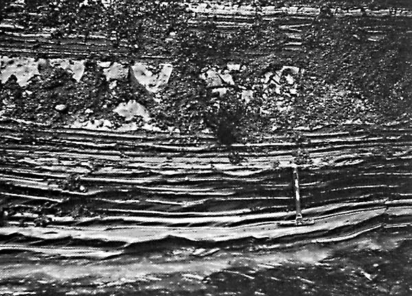
Figure 9-22a, modified from Strahler (1960), shows the landforms associated with glacial, glaciofluvial, and glaciolacustrine processes at the margin of a glacier lobe of ice cap or ice sheets. Significant glaciofluvial ice-contact features include eskers and kames, but only the esker is large enough to be discernible on Landsat images (Slaney, 1981; Erling Lindstrom, 1985, written communication). Figure 9-22b is an oblique aerial photograph looking north-northwest across the prominent esker located in Rörströmssjön, a lake in northwest Ångermanland, Sweden. The principal ice-stagnation landform visible on Landsat images is the kettle, which is usually occupied by a lake. The most dominant proglacial landform is the outwash plain or sandur (Figure 9-22a). Proglacial lakes (Plate G-23) commonly form at the edge of a lobe of glacier ice or at the terminus of a valley or outlet glacier. Such lakes become the sites for the deposition of deltas. Proglacial lakes are also important in the study of glacial stratigraphy because of the record of multiple cyclical (annual) sedimentary laminar couplets, called varves (Figure G-23.2), which form on their bottoms. Ephemeral ice-dammed lakes are also common at the edges of valley glaciers.
| Figure 9.21. Characteristic morainal and other landforms resulting from glacial and fluvial deposition processes of a valley or outlet glacier (from Flint, 1971). |  |
|---|
Glacial lakes are a common landscape element of glaciated terrains, especially in areas covered by ground moraine (Plate G-17). A common glacial lake is one that forms from the damming of a valley by a moraine. Glaciers may also overdeepen a valley through erosion; after the glacier recedes or disappears, such valleys may be filled by lakes. If overdeepening occurs in a coastal area, an arm of the ocean may occupy the valley, forming a fjord (see Plate G-14).
As already noted, deltas are common features in proglacial lakes. Much larger deltas can also form in lakes downstream from an active glacier or along the coast or in fjords from the enormous load of sediment discharged in glacial meltwaters from the terminus of a glacier.
An ice sheet represents a large surplus mass on the Earth´s surface that may slowly depress the Earth´s crust at a ratio of about 3:1 (3000 m of ice will deform the crust about 1000 m). After the ice sheet disappears, the crust will slowly restore itself in an isostatic process called glacial rebound. Along deglaciated coastal areas, a complex relationship exists between eustatic rise in sea level caused by the restoration of water to the oceans, new loading of the crust by the addition of sea water, and rebound resulting from the unloading of glacier ice. In some areas, the record of this rebound is preserved in a concentric series of strand lines (see Plate C-23).
 |
 |
|---|
Figure 9.22a. Landforms associated with glacial and fluvial glacial deposition processes at the margin of a glacier lobe of an ice cap or ice sheet (from Strahler, 1960).
| Figure 9.22b.Oblique aerial photograph of esker in Rörströmssjön, northwest Ångermanland, Sweden (photograph by Erling Lindstrom). | 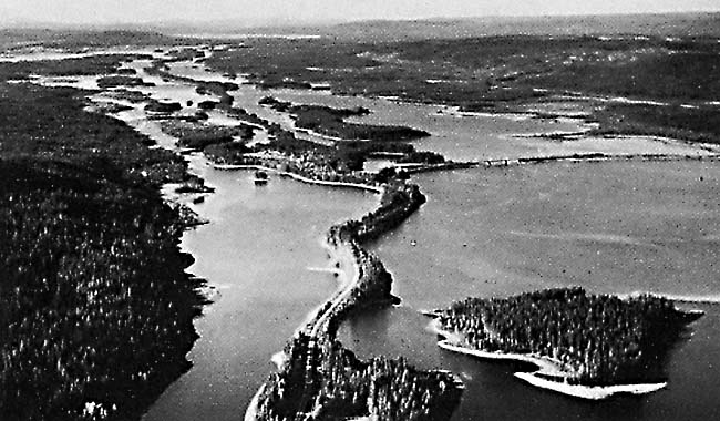 |
|---|
PERIGLACIAL LANDFORMS
Periglacial landforms (Embleton and King, 1975b) form in cold-climate environments at high latitudes, on high mountains, and in proximity to glaciers. Although a number of landforms are associated with ground ice, such as hummocks, palsen (Friedman, et al., 1971), pingos, thermokarst, patterned (polygonal) ground, and rock glaciers, only two of these have dimensions large enough to be discernible at the spatial resolution of the Landsat MSS image (79-m pixel): thermokarst (Svensson, 1983), and rock glaciers. Figure 9-23 shows raised-edge, ice-wedge polygons on the northern coastal plain of Alaska near Barrow. The diameters of the polygons are 7 to 15 m, well below the spatial resolution capability of the Landsat MSS image. Aufeis (naled or icing), large surficial deposits of ice, can also be delineated on Landsat MSS images (Sloan et al., 1976). Figure 9-24 is an August 4, 1975, Landsat MSS band 6 image showing aufeis (naled) remnants that formed during the previous winter along the drainages of the Kuparuk, Echooka, Ivishak, and Shaviovik Rivers, northeastern Alaska. Determination of other periglacial features common in a cold-climate environment is generally inferential, being derived from preexisting ancillary knowledge of the area encompassed by the Landsat image (Anderson et al., 1973). Thaw lakes (Table 9-7), special types of periglacial landforms resulting from thermokarst processes acting on perennially frozen ground or permafrost, are most evident on Landsat MSS images (Svensson, 1983) (Plate G-25). According to Péwé (1975), permafrost underlies about 20 percent of the land area of our planet and is especially widespread in the northern polar areas. Figure 9-25 shows the distribution of permafrost in the northern hemisphere (Péwé, 1975).
| Figure 9.23. Oblique aerial photograph of ice-wedge polygons on the northern coastal plain of Alaska. | 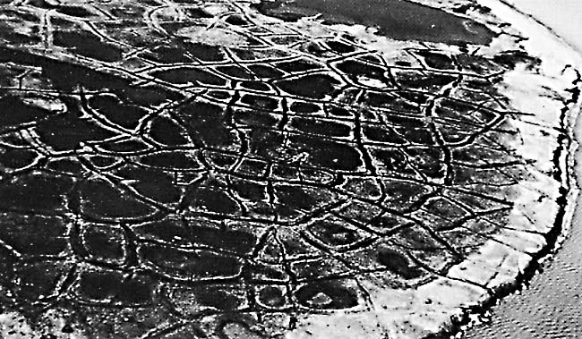 |
|---|
Editors Note:
Many of the glacial landforms, both erosional and depositional, and related features described in this introduction and shown in Figures 9-21 and 9-22 are difficult to pick out and identify in space imagery at Landsat-scale resolutions or less. Under the best of conditions, certain features are evident around active glaciers that are still producing them. Medial moraines on the glacial ice are easy to spot because of the sharp contrast between dark rock materials and bright ice, but lateral and terminal moraines, as well as kame terraces and some features in the outwash plains, are usually too small or dark or are lacking in relief to stand out. Deposits extending over wide regions covered by continental glaciers are frequently even more difficult to recognize despite their broad areal distribution. Even extensive terminal moraines are hard to discern unless they give rise to soils that display notably different spectral and physical properties. Eskers may appear conspicuous on the ground (Figure 9-22b) but seldom can be located, much less identified, even in glacial terrains where they may be commonplace. Drumlins, on the other hand, are often large enough in dimensions to be noted, especially where they occur in swarms (Plate G-19).
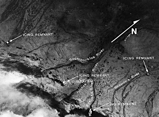 |
Figure 9.24. Landsat image of aufeis (naled) remnants (arrows) in northeastern Alaska. |
|---|
In addition to the foregoing factors (smallness, low relief, lack of contrast, and discontinuous distribution), vegetation cover (particularly in regions now heavily forested) and land-use practices (which effectively mask morainal features in much of the central and northern Great Plains) also prevent individual depositional features from being readily detected in Landsat imagery, even in some instances where they may predominate in a scene. As a rule, winter imagery is better for discriminating larger glacial features because the low Sun angle affords a natural enhancement as shadows call attention to small topographic differences (Plate G-15). Although snow cover may inhibit recognition of some smaller glacial landforms, in some instances it aids in highlighting certain features ("fingerprint dusting" effect). Features that possess sharp spectral contrasts with their surroundings normally show up better in summer imagery. (October is generally an optimum time to look for glacial features in parts of the northern hemisphere such as the Canadian Shield.)
| Figure 9.25.Map of permafrost distribution in the northern hemisphere (from Péwé, 1975). |  |
|---|
| Type | Formation | Features |
|---|---|---|
| Backwearing | By lateral erosion, by streams, lakes, or ocean | Gullies Thermocirques Thaw lakes Thermokarst mounds |
| Downwearing | By melting downward of ground ice. Usually develop as flat, shallow depressions in level areas. | Alases Thermokarst valleys |
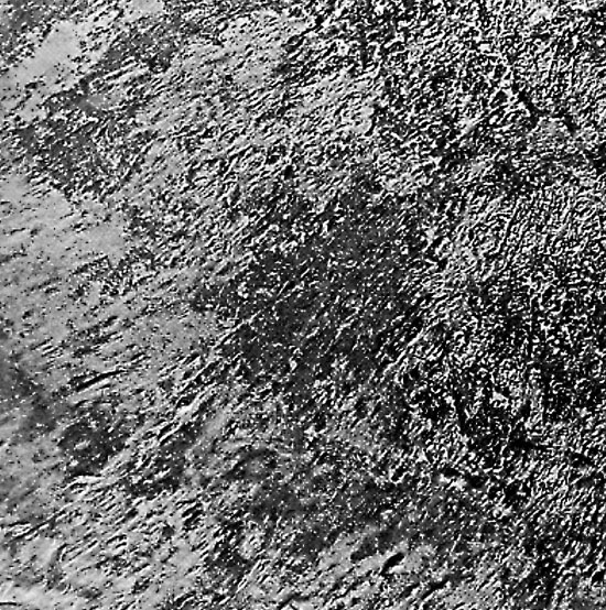
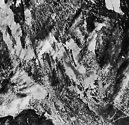
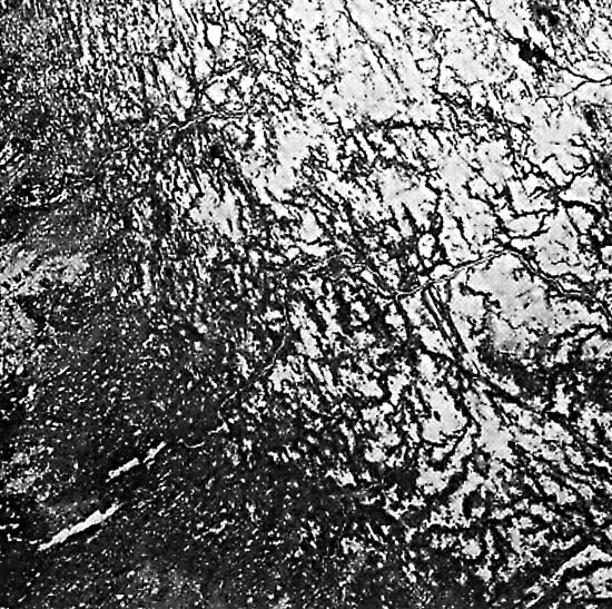
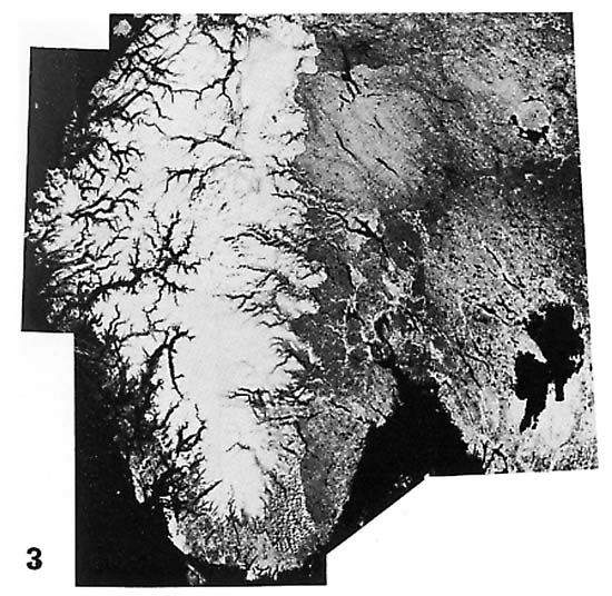
Landsat images (and mosaics therefrom) excel in providing synoptic information about one class of glacial features: aligned landforms and lineations imposed on the terrain by the passage of ice sheets across broad regions. Three Landsat images (interpreted by Canadian colleagues) illustrate this: In Figure 9-26a, showing a glaciated Precambrian surface in central Québec, a pronounced lineation oriented to the southwest is produced by large crag-and-tail hills (especially evident in the lower left), possibly mixed with drumlins. Large-scale glacial fluting in Manitoba is emphasized in Figure 9-26b by ice formed in lakes and wetlands in the furrows; the direction of ice movement is obvious. Two directions of motion are evident in Figure 9-26c, a scene in Ontario south of Hudson Bay. In the right half of the image, mega-grooves running nearly north-south appear to be fluting (and possible iceberg gorge marks) in a flatlands composed of Paleozoic marine deposits. Pronounced northeast-southwest lineations in glacial cover over Precambrian bedrock in the left half of the image also appear to be glacial scouring effects that localize elongate lakes.
| Figure 9.26a | Figure 9.26b | Figure 9.26c |
|---|---|---|
 |
 |
 |
Continue to Plate G-1| Chapter 9 Table of Contents.| Return to Home Page| Complete Table of Contents|