Now that we have seen the individual Landsat Thematic Mapper (TM) bands and color composites that show our study image, we need to investigate the power of two of the most common image processing routines for improving scene quality. These routines fall into the descriptive category of Image Enhancement or Transformation. We used the first image enhancer, stretching, on all the TM images we have looked at so far, to improve their quality for this tutorial. Different stretching options are described next. We will evaluate the other routine, filtering, shortly.

Contrast stretching involves altering the distribution and range of DN values. A casual viewer and an expert usaully conclude from direct observation that modifying the range of light and dark tones (gray levels) in a photo or a computer display is often the singlemost informative and revealing operation performed on the scene. When carried out in a photo darkroom during negative and printing, the process involves shifting the gamma (slope) or film transfer function of the plot of density versus exposure (H-D curve). This is done by changing one or more variables in the photographic process, such as , the type of recording film, paper contrast, developer conditions, etc. Frequently the result is a sharper, more pleasing picture, but certain information may be lost through trade-offs, because gray levels are "overdriven" into states that are too light or too dark.

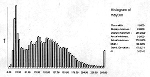
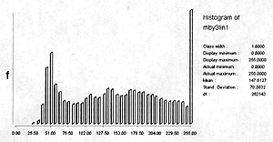
Contrast stretching by computer processing of digital data is a common operation, although we need some user skill in selecting specific techniques and parameters (range limits). For Landsat data, the DN range for each band, in the entire scene or a large enough subscene, is calculated and displayed as a histogram (recall the histogram for TM band 3 of Morro Bay). Commonly, the distribution of DNs (gray levels) can be unimodal and may be Gaussian (distributed normally with a zero mean), although skewing is usual. Multimodal distributions (most frequently, bimodal but also polymodal) result if a scene contains two or more dominant classes with distinctly different (often narrow) ranges of reflectance. Upper and lower limits of brightness values typically lie within only a part (30 to 60%) of the total available range. The (few) values falling outside1 or 2 standard deviations may usually be discarded (histogram trimming) without serious loss of prime data. This trimming allows the new, narrower limits to undergo expansion to the full scale (0-255 for Landsat data). Linear expansion of DN's into this full scale is a common option.

Other stretching functions are available for special purposes. These are mostly nonlinear functions that affect the precise distribution of densities (on film) or gray levels (in monitor image) in different ways, so that some experimentation may be required to optimize results. Commonly used special stretches include:1) Piecewise Linear, 2) Logarithmic, 3) Ramp Cumulative Distribution Function, 4) Probability Distribution Function, and 5) Linear with Saturation. Histogram Equalization is a stretch that favorably expands some parts of the DN range at the expense of others by dividing the histogram into classes containing equal numbers of pixels. For instance, if most of the radiance variation occurs in the lower range of brightness, those DN values may be selectively extended in greater proportion to higher (brighter) values.

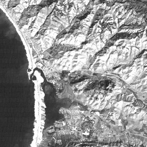
To illustrate contrast stretching (also called autoscaling) we apply the IDRISI STRETCH function to band 3. Recall that the histogram (see above) of raw TM values shows a narrow distribution that peaks at low DN values. We might predict from this that we have a dark, flat image. This is indeed the case:

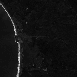
Most of the DN values, however, lie between 9 and 65 (there are values up to 255 in the original scene but few of them). We can perform a simple linear stretch so that 9 goes to 5 and 65 goes to 255, with all values in between getting stretched proportionately. Next we show this expanded histogram, and next to it, is the resulting new image.

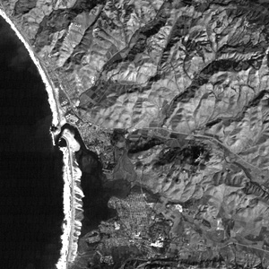
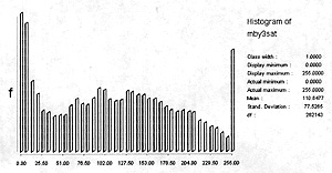
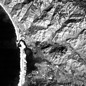
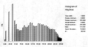
Now, most of the scene features are discriminable. But the image still is rather dark. Lets try instead to choose new limits in which we take DNs between 5 and 45 and expand these to 0 to 255. This stretch results in the following histogram and image:

The histogram for this image is polymodal, with a lower limit near 25 and a large number of DN pixels at or near 255. This accounts for the greater scene brightness (light tones).

Next we try a Linear-with-Saturation stretch. Here we assign the 5% of pixels at each end (tail) of the histogram to single values. The consequent histogram and image are:

The image appears as a normal and pleasing one, not much different from the others. But, comparing this one with either of the linear-stretched versions shows that real and informative differences did ensue.

Finally, we carry out a Histogram Equalization stretch, with these results:

The image is similar to the Saturation version. Note that pixel frequencies are spread apart at low DN levels and (closely-spaced) at high intervals.

Let us reiterate. Probably no other image processing procedure or function can yield as much new information or aid the eye in visual interpretation as effectively as stretching. It is the first step, and most useful function, to apply to raw data.

1-12: Comments have been made above about the relative quality and information content of each of the stretches displayed. In your opinion, which seems best and is most pleasing to the eye. ANSWER

Collaborators: Code 935 NASA GSFC, GST, USAF Academy
Contributor Information
Last Updated: September '99

Webmaster: Bill Dickinson Jr.
Site Curator: Nannette Fekete
Please direct any comments to rstweb@gst.com.