We turn now to a final consideration of some geomorphic properties that apply to the entire study area. We made a map showing relief relative to terranes from digitized data in the Digital Elevation Map 1:250,000 sheet for the Klamath Mountains:

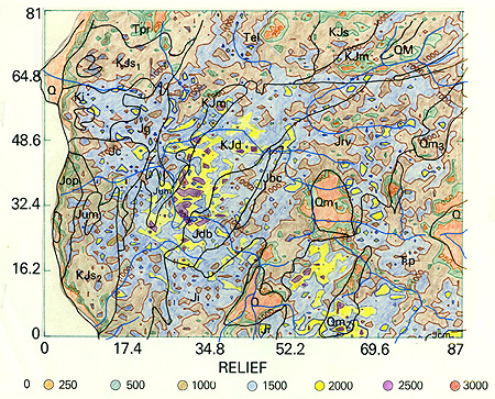
Maximum relief occurs in the central Yolla Bolly terrane. This is also the area (in purple) of highest maximum elevations (1,174 m [3,850 ft]). This height and the ease of downcutting into the shales account for the relief. We show the lowest inland areas in orange-red. These areas are valleys, one containing Grants Pass, the largest town in the Klamaths, that Quaternary deposits cover. The Grant Pass valley is underlain in part by a granitic rock, which weathers into a thick "rotten rock" (saprolite) soil and erodes easily to leave a lowlands.

At this point, with some trepidation, we introduce the concept of hypsometery. We treat this rather complicated idea in a general way because, when we applied it to the Klamath terranes, some interesting results ensued (but their significance remains unclear).

Hypsometry refers to finding the distribution of elevations as a function of area occupied by each contour interval within some geographic unit (such as a topographic sheet). This process determines the fraction of a surface bounded by specified elevations. These diagrams (from Process Geomorphology, by D.F. Ritter) depict the concept:

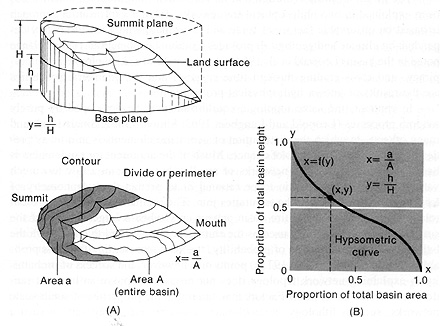
We define the calculation unit as a volume bounded by the base and summit planes, of a given area A, and the total height (H) from the base to the highest elevation. As we move from the lowest elevation (base) upwards on the map progressively through increasing values of h, we measure all the areas within each contour interval. With each successive increase in h, the area increases by some new value of a. This progression is cumulative. When plotted on an x-y diagram, the relative values of h/H and a/A form the hypsometric curve (center right). Note that x and y values are dimensionless, representing proportions of the total area and height. Thus for y = 0, all heights are above the datum plane and therefore, lie within the total area, i.e., x = 1. We can calculate the area below the curve as the hypsometric interval (HI). As applied to a drainage basin, HI represents the unconsumed volume as a percentage delimited by base plane, summit plane, and perimeter area.

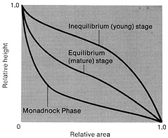
Various factors influence the shape of the hypsometric curve and its position in the x-y plot–hence its HI value. Direct interpretation of a family of curves, and their possible interrelationships, is not straightforward, but we can make some generalizations. Overall, the HI broadly denotes the degree of uplands dissection. Look at the bottom diagram above. Its top curve can typify a relatively high terrain (keep in mind that the geomorphic unit, the drainage basin, consists of valleys and intervening divides and all slopes in-between), which may be in the early stages of downward erosion and slope wall development. The lower curve is characteristic of the late stage of erosion, marked by broad, low valleys, with occasional higher promontories ("monadnocks"). Of course, various combinations of surfaces can lead to similar curves in proximate positions.

Again, using digitized topographic data, we produced hypsometric curves for individual Klamath terranes and, for several segments thereof. We show hand plots of these segments in the top diagram, and plots for the three aforementioned Yolla Bolly segments are on the bottom.

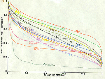
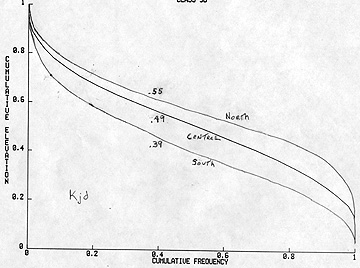
We do not ask you to grasp in detail the relations among these curves (it is hard to identify some of the terrane symbols), because we have not derived specific interpretations that have obvious meaning. Suffice to comment that the one on top associates with the sliver of Briggs Creek terrane, which is one of the highest. The Jj (Smith River) and Jdb (Dry Butte) terranes also have high elevations and rugged topography. But, the Yolla Bolly terrane as a whole (KJd in the top diagram) occupies a lower position in the set of plots. From the bottom diagram, it is evident that there is moderate variation within this terrane, although less than the range among all terranes in the top diagram. The three map units–none are actual terranes–with the lowest curves (and thus smallest HI's) are the lowlands associated with the Quaternary coastal plains and inland areas, and the granite lowlands.

When we plot the values of HI (in fractions of 1.00) on the terranes map, a pattern emerges.

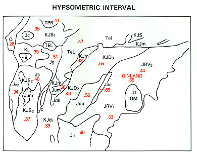
The highest values of HI cluster in the central terranes. This pattern suggests that these are also topographic units that have not been significantly downcut towards sea level. Those units near the coast, with lower elevation levels, even though younger (docked later), may have eroded more completely. Although, because their stream heights and gradients are closer to sea level, we expect a smaller amount of relief. But, we stop here without further explanation, because the hypsometric data, while tantalizing, are not equivocally interpretable.

Collaborators: Code 935 NASA GSFC, GST, USAF Academy
Contributor Information
Last Updated: September '99

Webmaster: Bill Dickinson Jr.
Site Curator: Nannette Fekete
Please direct any comments to rstweb@gst.com.