
We turn now to lineaments. In the early days of Landsat, perhaps the most commonly cited use of space imagery in Geology was to detect linear features that appeared as tonal discontinuities. Almost anything that showed as a roughly straight line in an image was suspected to be geological. Most of these lineaments were attributed either to faults or to fracture systems that were controlled by joints (fractures without relative offsets). Lineaments are well-known phenomena in the Earth's crust. Rocks exposed as surfaces or in road cuts or stream outcrops typically show innumerable fractures in different orientations, commonly spaced fractions of a meter to a few meters apart. These lineaments tend to disappear locally as individual structures, but fracture trends persist. The orientations are often systematic meaning, that in a region, joint planes may lie in spatial positions having several limited directions relative to north and to horizontal. For example, 60% of the joint planes might fall into a cluster of fractures with azimuths between N40W and N60W and inclinations between 30 and 40 degrees).
Where continuous subsurface fracture planes that extend over large distances and intersect the land surface produce linear traces (lineaments). A linear feature in general can show up in an aerial photo or a space images as discontinuity that is either darker (lighter in the image) in the middle and lighter (darker in the images) on both sides; or, is lighter on one side and darker on the other side. Obviously, some of these features are not geological. Instead, these could be fence lines between crop fields, roads, or variations in land use. Others may be geo-topographical, such as ridge crests, set off by shadowing. But those that are structural (joints and faults) are visible in several ways. They commonly are opened up and enlarged by erosion. Some may even become small valleys. Being zones of weak structure, they may be scoured out by glacial action and then filled by water to become elongated lakes (the Great Lakes are the prime example). Ground water may invade and gouge the fragmented rock or seep into the joints, causing periodic dampness that we can detect optically, thermally, or by radar. Vegetation can then develop in this moisture-rich soil, so that at certain times of year linear features are enhanced. We can detect all of these conditions in aerial or space imagery.
When we illuminate a space image, particularly a transparency on a light table, we can often spot numerous linear or boundary discontinuities that we can record on tracing paper. The resulting lineaments map may have dozens, even hundreds of straight or slightly curved lines. But, scientific skepticism can raise key questions: Are they real? Do they all correspond to the same feature or phenomenon? If not, what is the proper identity of each one? And, finally, how do we verify their existence and determine their identities? These are important issues since we know lineaments (particularly faults) play key roles in location minerals and some oil or /gas deposits. They may also give clues to structural activities that bear on earthquakes. We save responses to these queries until the end of this section, after we cover how lineaments appear in images. Near the end of Section 5, we will again consider how human operator variations affect the correctness and consistency in picking valid lineaments amidst phony lines.
The very first practical use of ERTS-1 (Landsat-1) imagery in any discipline was the drawing by Dr. Paul D. Lowman, Jar, of a geologic structures map from the first color composite image. He is a geologist at Goddard Space Flight Center, and an expert on space photography (he prepared Section 12 on Astronaut Imagery in this tutorial). The image was of the central California coast around Monterey Bay, acquired 3 days after launch. This map confirmed
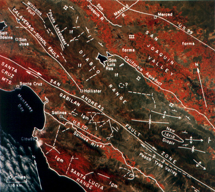
predictions from his studies of astronauts' photos that Landsat would be an efficient tool for recognizing faults and other known structural trends in small-scale imagery. Inspite of lower resolutions, these images excel in portraying regional geologic settings and are easily modified by digital processing. Within a month of the Landsat launch, images of the central Rocky Mountains were delivered to a team of investigators at the University of Wyoming.
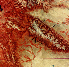
On this team, Professor Ronald Parker, a structural geologist, had been field mapping lineaments and other deformation features in the Wind River Mountains in the west-central part of the state. This great block of metamorphic and igneous basement rocks, flanked and patchily-covered by Paleozoic sedimentary rocks, is part of a segment of the Rockies where sections of the crust had been uplifted six km or more above other segments. Other segments stayed put or had downdropped to form deep (up to six km below the present surface) basins now back-filled by erosional debris from the surrounding mountain groups. As shown here by this Landsat image, the Wind River Mountains (center right) lie between the Wind River Basin (upper) and Green River Basin (lower), with the Gros Ventre and Hoback Ranges to the west. The Wind River Mountains rise to more than 3940 m (13,000 feet) above sea-level and have been strongly dissected by rivers and glaciers that exposed and carved many major faults and lineaments. We can easily map most of these lineaments in the field or from the limited aerial photos. As part of the project, NASA had previously flown a U-2 on a single pass, taking pictures of terrains similar to our next image. This photo shows an eroded granitic surface with numerous lineaments.
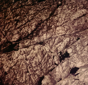
2-15: Do you know the difference between a fault and a fracture? How might the two types be separated visually on an aerial photo or space image? ANSWER
2-16: The above aerial photo displays lots of faults and fractures - a real hodgepodge. Can you think up a good way to separate them and show their relative orientations as well as the relative number in any given direction? ANSWER
Dr. Parker, during five field seasons (camping in the high country, and supported by pack mules, ) had completed ground mapping faults, shear zones, and filled dikes in about 20% of the Wind River uplifted block. He supplemented his work by photointerpretating the U-2 strip. His map is shown below on the left.
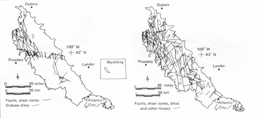
Upon receipt of a band 5 Landsat (ERTS) image, he produced the lineaments map on the right in just three hours (including a break). Some of the newly plotted lineaments had been discovered earlier by other geologists, but most were heretofore unknown, and some of those have since been verified in the field. This great breakthrough effort now meant that we could map the synoptic overview of a large section of fractured continental crust with acceptable reliability in less than a day rather than months of difficult field work in poorly accessed terrain. This new method also meant great savings in time and money.
But, this mapping is of necessity incomplete and somewhat misleading. The maps below compare the ERTS and Skylab (Mission S-190B) Lineaments maps
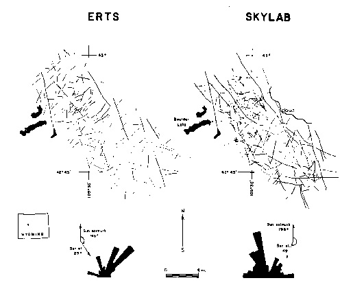
from the central Wind River Mountains. We plotted the orientation (azimuth or compass bearing) of the dominant direction relative to north, of each linear feature in a rose diagram (at the bottom of the map). This diagram shows directions for all linear sets that we grouped in intervals (here 10 degrees), such that the length of the tapering bar in each interval is proportional to its frequency distribution (relative proportion) among all lineaments in the intervals distributed over the 180 degrees; that encompass west to east trends. Note that the dominant directions for ERTS lineaments are NE, whereas those for Skylab are NNW.
The cause of this difference between the two observations is simply time-of-day. The ERTS image was acquired around 10:30 A.M., local time, when the Sun's rays came from a SE position at a moderate elevation angle. Fractures occupying depressions that trend NE are shadowed on their NW side, and hence, stand out in the image as shadow relief. Whereas, those trending NW are equally illuminated on both sides and hence largely invisible and easily missed. On the other hand, the Skylab photo was taken in mid-afternoon, when the Sun was shining towards the NE at a higher elevation, so that shadows would maximize along NW trending lineaments. This illumination bias is a well-known effect (see Section 11) and forces us to decide cautiously about structural trends when only data sets taken at one time of day are available. The obvious solution is to use multiple data sets, obtained at different times. Unfortunately this is not an option with Landsat. However, a geostationary satellite that can image at any time would circumvent this problem, but no high resolution systems [superior to meteorological ones] are operational yet.
2-17: How could you get around (overcome) this time of day or sun angle bias, using a satellite(s)? ANSWER

Collaborators: Code 935 NASA GSFC, GST, USAF Academy
Contributor Information
Last Updated: September '99
Webmaster: Bill Dickinson Jr.
Site Curator: Nannette Fekete
Please direct any comments to rstweb@gst.com.